Image Segmentation
1 | import cv2 |
1 | def showImage(image): |
1 | img = cv2.imread('IMG_0377_o.JPG', cv2.IMREAD_COLOR) |

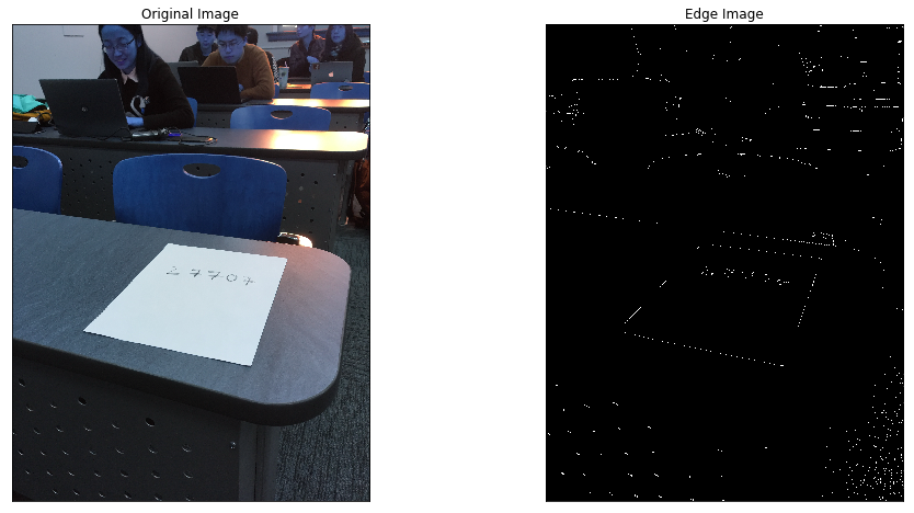
Use the Canny Algorithm in OpenCV to extract the edges
Canny algorithm is applied to extracted edges in this image, then the edges can be use to local contours
1 | edges = cv2.Canny(img,200,240) |
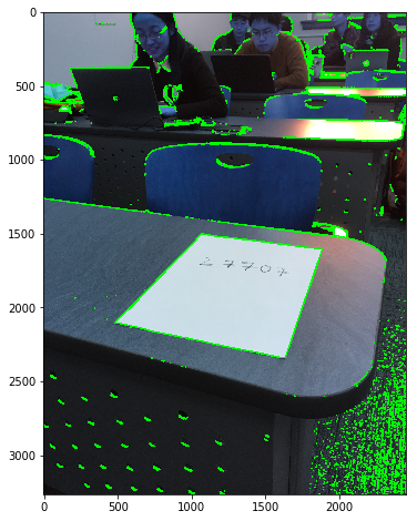
Find countours based on the edges extracted from image
Edges found by canny is used to find contours of this images, from the images showed belowed we can see that a lot of contours are extracted from the image.
1 | im2, contours, hierarchy = cv2.findContours(edges, cv2.RETR_EXTERNAL , cv2.CHAIN_APPROX_SIMPLE) |
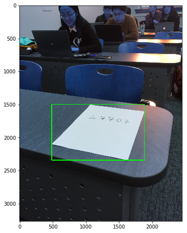
Find the Max Contor with largest contour area
For this problem, the white paper sheet in this image has the largest contour, we can extracted the contour of this white paper sheet by finding the largest contour.
1 | c = max(contours, key = cv2.contourArea) |
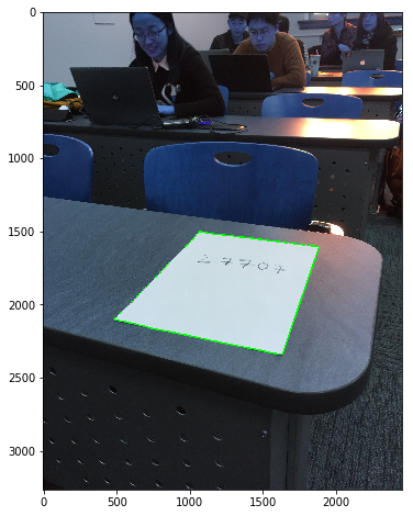
Approximate the Contor
After finding the contour of this white paper sheet, we can use Geometric shape such as rectangle or polygon to approximate this countour. From the result showed belowed, we can see that polygon did well in the shape approxiamtion.
rectangle approximation
1 | imcopy = img.copy() |
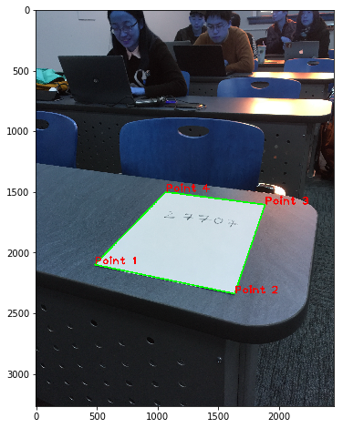
Polygon approximation
By applying polygon approximation, the 4 coner points was extracted, which can be used in the later experiment of perspective transformation.
1 | epsilon = 0.01*cv2.arcLength(c,True) |
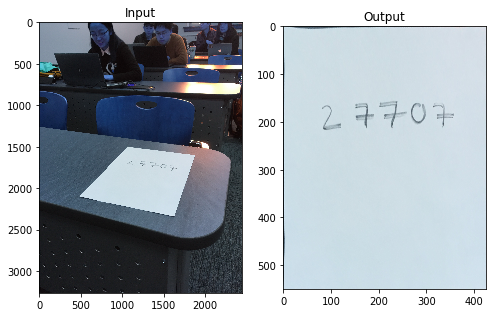
Applied Perspective Transformation
- Projective transformation(Perspective transformation) is the combination of affine transformation and projective wrap.
Suppose(x, y, 1) is a point in homogeneous coordinate. The projective transformation of this point is as followed.
This 8 parameters matrix maps point$(x,y,1)$ in one projective to point $(x’/w’,y’/w’,1)$ in another projective.
We can get 2 equations from one point mapping, to solve this 8 parameter tranformation equation, we need more than 4 points mapping. When this tranformation equation be solved, can can applied it to get a new image.
1 | imcopy = img.copy() |
Build a CNN model with tensorflow
1 | import tensorflow as tf |
1 | from tensorflow.examples.tutorials.mnist import input_data |
1 | def weight_variable(shape,name): |
1 | def conv2d(x, W): |
1 | def create_placeholders(n_x=784, n_y=10): |
1 | def initialize_parameters(): |
1 | def forward_prop(x, keep_prob, parameters): |
1 | tf.reset_default_graph() |
1 | num_epochs = 16 |
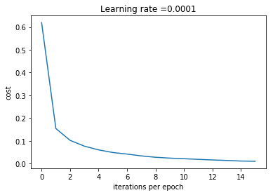
Parameters have been trained!
test accuracy 0.9927
Save the parameters to local data
Because the CNN model takes a long long time to train, thus it will save time if we can save the trained parameters to a local file
1 | import pickle |
Load data from saved file
1 | testparams = pickle.load(open("params.pkl","rb")) |
1 | def predict(x, parameters): |
1 | def forward_propagation_for_predict(x, parameters): |
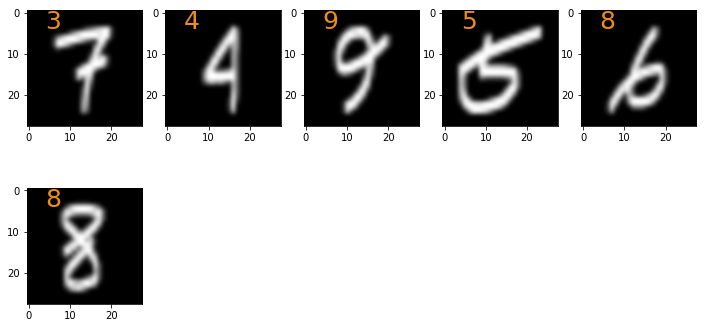
Experiment of Self-Written Digits Image
1 | import cv2 |
1 | img = cv2.imread('test_digit4.png', cv2.IMREAD_COLOR) |
1 | plt.figure(figsize=(10,5)) |
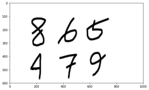
1 | blur_img = cv2.GaussianBlur(img, (5,5), 0) |
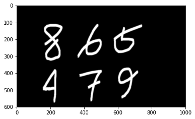
1 | ret,thresh = cv2.threshold(img,127,255,cv2.THRESH_BINARY_INV) |
1 | plt.imshow(thresh, cmap = 'gray', interpolation = 'bicubic') |
1 | def generateImage(small): |
1 | images = [] |
1 | fig=plt.figure(figsize=(12,4)) |
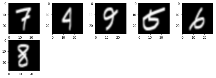
Test my Own hand written
1 | fig_out=plt.figure(figsize=(12,6)) |